Data Visualisation Plugins
This page is intended to describe how to use the available visualisation plugins with the existing gCube infrastructure.
Contents
GeoExplorer Plugins
These plugins are intended to extend the GeoExplorer functionality by adding some extra visualisation options (e.g. feature filtering, feature subsets visualisation)
Interactive Layers
The specific component exists since the 2.14 gCube release, by the name InteractiveLayers.
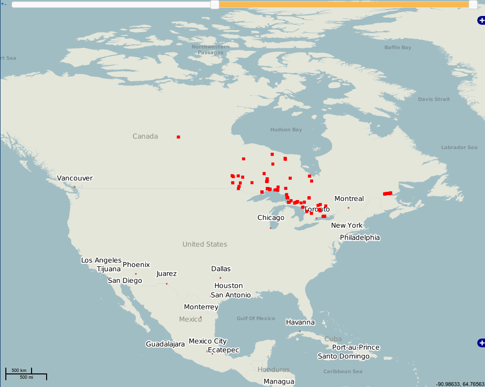
Layer with time filtering
This is an extended version of the Layer class (gwt-openlayers-client) which GeoExplorer already uses.
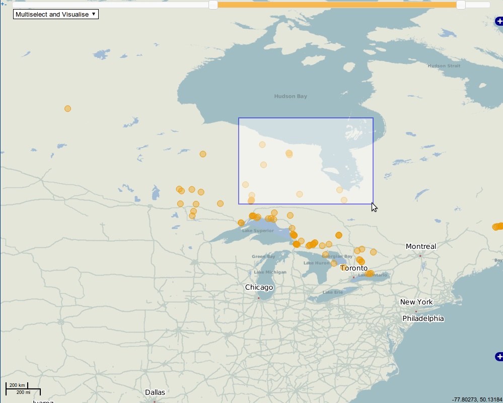
The layer, is altered to contain a double slidebar (a JQuery-UI slidebar), which filters the content of the layer on the given time window.
The layer upon it's initialization needs to have the following information:
- the layer name (within the GeoNetwork)
- the workspace name under which the layer resides
- the geoserver location (URL).
- a unique id for the slidebar of the layer (could be same as the layername)
- the Date field name of the layer by which the time filtering will be done.
- a "from" Date
- a "to" Date
WMS Layer
The constructor is:
Layer OpenLayers.createInteractiveFilterLayerWMS(String serverWmspath, String workspace, String layerName, String slidebarID, String dateColumnName, Date startDate, Date endDate)
where 'startDate' is the minimum date for the filter slider and 'endDate' the maximum date
Thus, a call
Layer barLayer = OpenLayers.createInteractiveFilterLayerWMS("http://geoserver2.d4science.research-infrastructures.eu/geoserver/wms", "timeseriesws" , "animalia_fishbase", "layerSlider", "datecollected", startDate, endDate);
where startDate and endDate are java.util.Date objects
will initiate a WMS Layer mapped to the underlying data with a slidebar within.
The serverWmspath, layername and workspace variables should all be known within the running scope !
It can be used by creating a instance of this modified layer instead of the default and adding it on the map.
Layer barLayer = OpenLayers.createInteractiveFilterLayerWMS("http://geoserver2.d4science.research-infrastructures.eu/geoserver/wms", "timeseriesws" , "animalia_fishbase", "layerSlider", "datecollected", startDate, endDate);
map.addLayer(barLayer);
Then, the layer reforms itself as user interacts with the slider.
WFS Layer
The constructor is:
Layer OpenLayers.createInteractiveFilterLayerWFS(String serverWmspath, String workspace, String layerName, String slidebarID, String dateColumnName, Date startDate, Date endDate)
where 'startDate' is the minimum date for the filter slider and 'endDate' the maximum date
Thus, a call
Layer barLayer = OpenLayers.createInteractiveFilterLayerWFS("http://geoserver2.d4science.research-infrastructures.eu/geoserver/wfs", "timeseriesws" , "animalia_fishbase", "layerSlider", "datecollected", startDate, endDate);
where startDate and endDate are java.util.Date objects
will initiate a WFS Layer mapped to the underlying data with a slidebar within.
The serverWfspath, layername and workspace variables are assumed to be known within the running scope !
It can be used by creating a instance of this modified layer instead of the default and adding it on the map.
Layer barLayer = OpenLayers.createInteractiveFilterLayerWFS("http://geoserver2.d4science.research-infrastructures.eu/geoserver/wfs", "timeseriesws" , "animalia_fishbase", "layerSlider", "datecollected", startDate, endDate);
map.addLayer(barLayer);
IMPORTANT note: dateColumnName should be of type "Date" and not "String" in the geoserver !
Advanced Layer Visualisations
In order to add the advanced visualisations on a layer, the modified (gwt-openlayers-client) Control class should be used.
Two different Control class versions are available - one for each Layer type, because of the different way data is requested on WMS and WFS.
The controls are initialized and added to the map similarly to the layer, needing only two inputs, the modified Layer object described previously and a String containing the type(s) of the advanced visualizations to enable.
Currently, there are the following types of advanced visualization available:
- Bubble plots for WMS layers
- Cumulative plots for WMS layes
- Timelines for WFS layers
WMS Layer Control sample initialization code
Control featureControl = OpenLayers.createWMSFeatureControl(barLayer, VisualisationTypes.allWMS());
map.addControl(featureControl);
the above code will add to the barLayer (which should be a WMS layer), a control with allWMS visualizations enabled.
WFS Layer Control sample initialization code
Control featureControl = OpenLayers.createWFSFeatureControl(barLayer, VisualisationTypes.allWFS());
map.addControl(featureControl);
the above code will add to the barLayer (which should be a WFS layer), a control with allWFS visualizations enabled.
It should be noted that the Layers are fully functional without the controls. The controls just add the advanced visualisations.
Species migration visualisation
Under construction
Standalone Components
These components are intended for generic use within the portal.
Quantitative properties visualisation
Component exists since the 2.13 release, by the name QuantitativePropertiesVisualisation
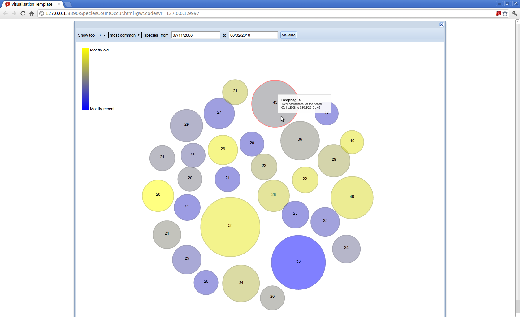
This is a generic component which is intended to provide a visualisation of a two or three dimentional vector sets.
The initial drive was to visualise marine species occurrencies, so the input set contained features {SpeciesID, number of occurences, skewness of the dates distribution}, however, it can be used to visualise feature sets with similar semantics.
This visualisation is served within GXT widgets, which currently are of the following types:
- Panel
- PopupPanel
- Dialog
- Window
The widget contains
- a control panel - to set some desired properties before querying the geoserver for the data (WFS protocol).
- a drawing canvas, in which the visualisation is shown.
The above widgets can be initiated by the following two constructors:
- (String layerName, String id, String name, String property1, String property2, int width, int height)
- (String geoserverUrl, String workspace, String layerName, String id, String name, String property1, String property2, int width, int height)
where
- layerName the layer as it is named in any geoserver,
- geoserverUrl is the url of a specific geoserver known to contain the layer
- workspace the workspace in which the layer belongs
- id is a unique id for the HTML div object of the created div panel,
- name, property1 and property2 are the naming of the three properties within the input data string (which is expected to be in GeoJSON form)
- width is the widget's initial width
- height is the widget's initial height
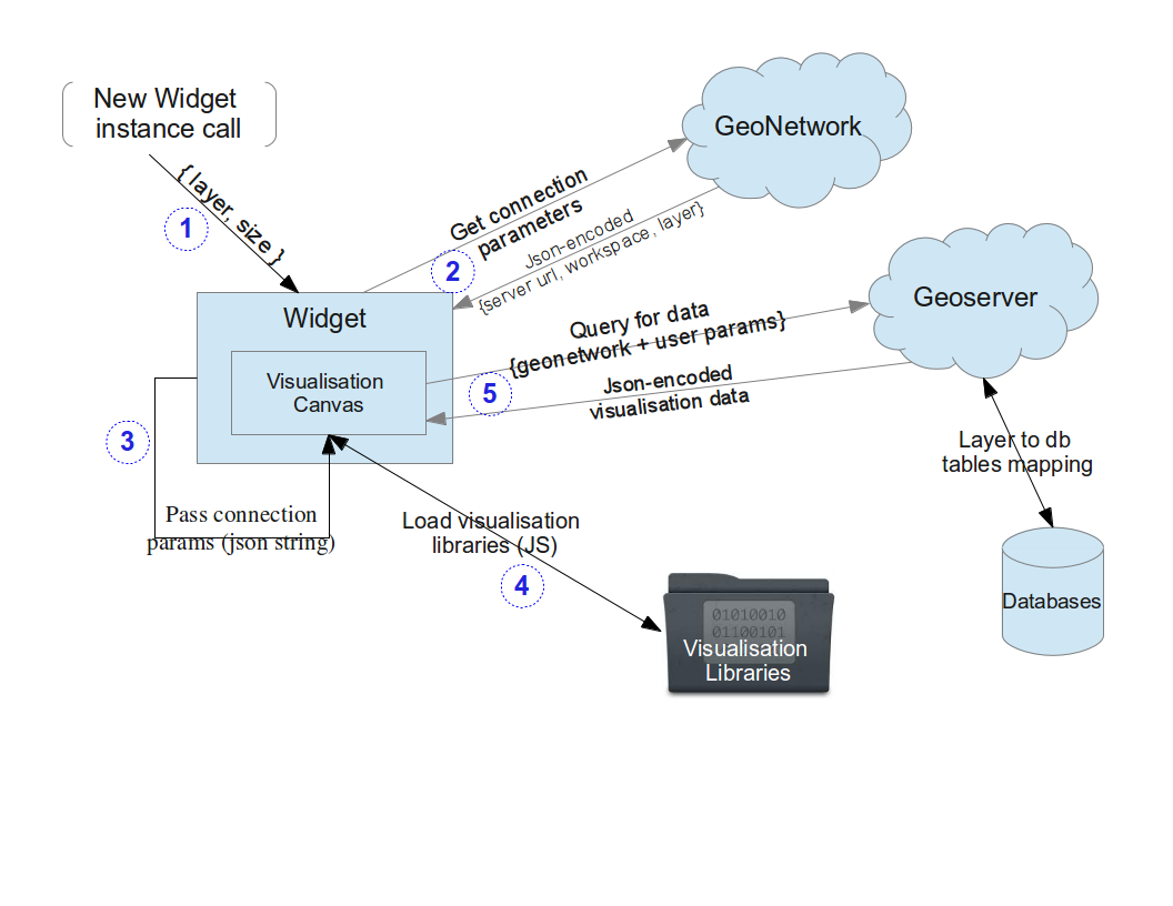
in the first case, the widget queries the geonetwork (using the geoserverinteface component) by the layer name, to find the connection parameters to the specific layer
in the second case, the geoserverURL, the workspace and the layer name are provided, so it contacts directly the layer to get the data
Thus, a Panel (1000x800) widget can be initiated by
BubblePlotPanel bpp = new BubblePlotPanel("layerABC", "bubbleplotdivID", "name", "occurrencies", "skewness", "1000", "800");
The above widgets need to get aggregated data (that is the occurrences and the skewness of the dates distribution), which should be computed by the layer and it's underlying infrastructure prior returning them to the widget.
An example follows to demonstrate the preprocessing needed in order to be able to use such a visualisation.
Assuming that a geoserver contains a datasource with 100 properties for each object e.g: {id, species_name, date_viewed, depth, longitude, latitude, fao_area, ... etc} and we want to visualise some quantitative properties. First step is to identify within the datasource, which are the quantitative properties which could be visualised. In this case, the name could be the species_name, the first property could be the count(species_name) and the second property could be the skewness(date_viewed).
The geoserverinterface should be used to programmatically create a layer linked to this datasource which will contain also a query to the datasource of the type "select species_name as name, count(species_name) as occurrencies, skewness(date_viewed) as skewness ....."
After creating the layer, it will output the values {name,occurrencies,skewness} which we will use upon the creation of the visualisation widget BubblePlotPanel (String layerName, String id, String name, String property1, String property2, int width, int height) e.g. BubblePlotPanel bpp = new BubblePlotPanel ("aVisualisationLayer", "visualisationwidgetID", "name", "occurrencies", "skewness", 1000, 800);
Because of all the preprocessing needed on the layers prior using the above widgets, a new widget which visualises directly a given GeoJSON encoded string rather than contacting any data source was created.
It is a GXT FramedPanel BubblePlotCanvas(String dataJSON, String idFieldName, String populationFieldName,String skewFieldName, String divID, String width, String height)


