Signal Processing

Signal Processing is a set of facilities that aim to analyze signals, or measure time-varying or spatially varying physical quantities. It is part of the gCube system facilities for Data Mining and Processing. It is especially used in order to to discover seasonality and periodicities in time series of observations. Such observations can refer to catch statistics, species presence occurrence or environmental parameters modulations. The Signal Processing facilities are included in the Ecological Engine gCube library. Such library is responsible for hosting all the basic data processing and mining for on biological and environmental datasets. The Signal Processing facilities especially aim at facing the following issues:

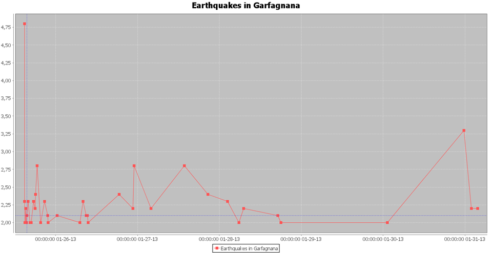
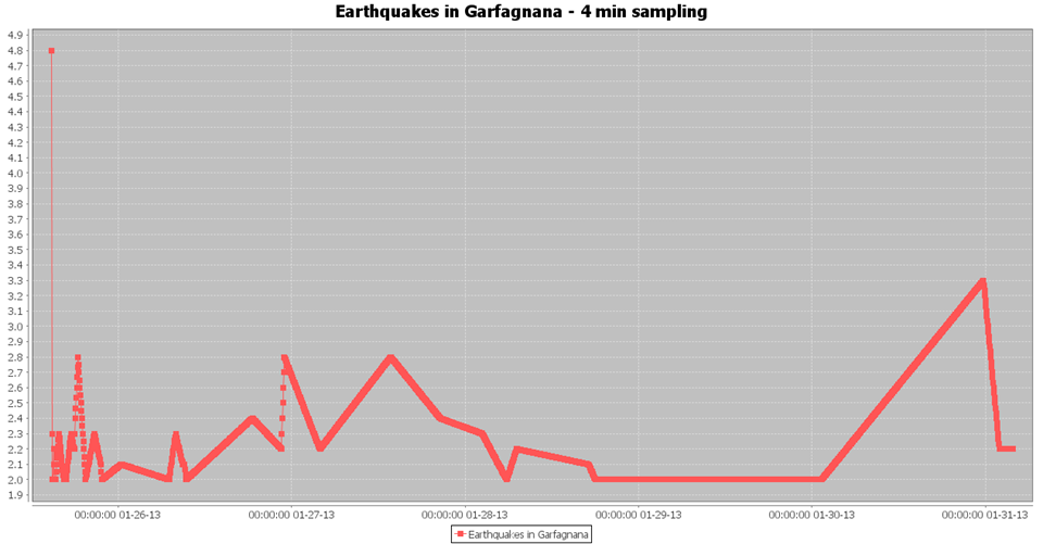
• Reconstruct a uniform sampled time series from a non-uniform time series
• Perform Short-Time Standard Fourier Analysis
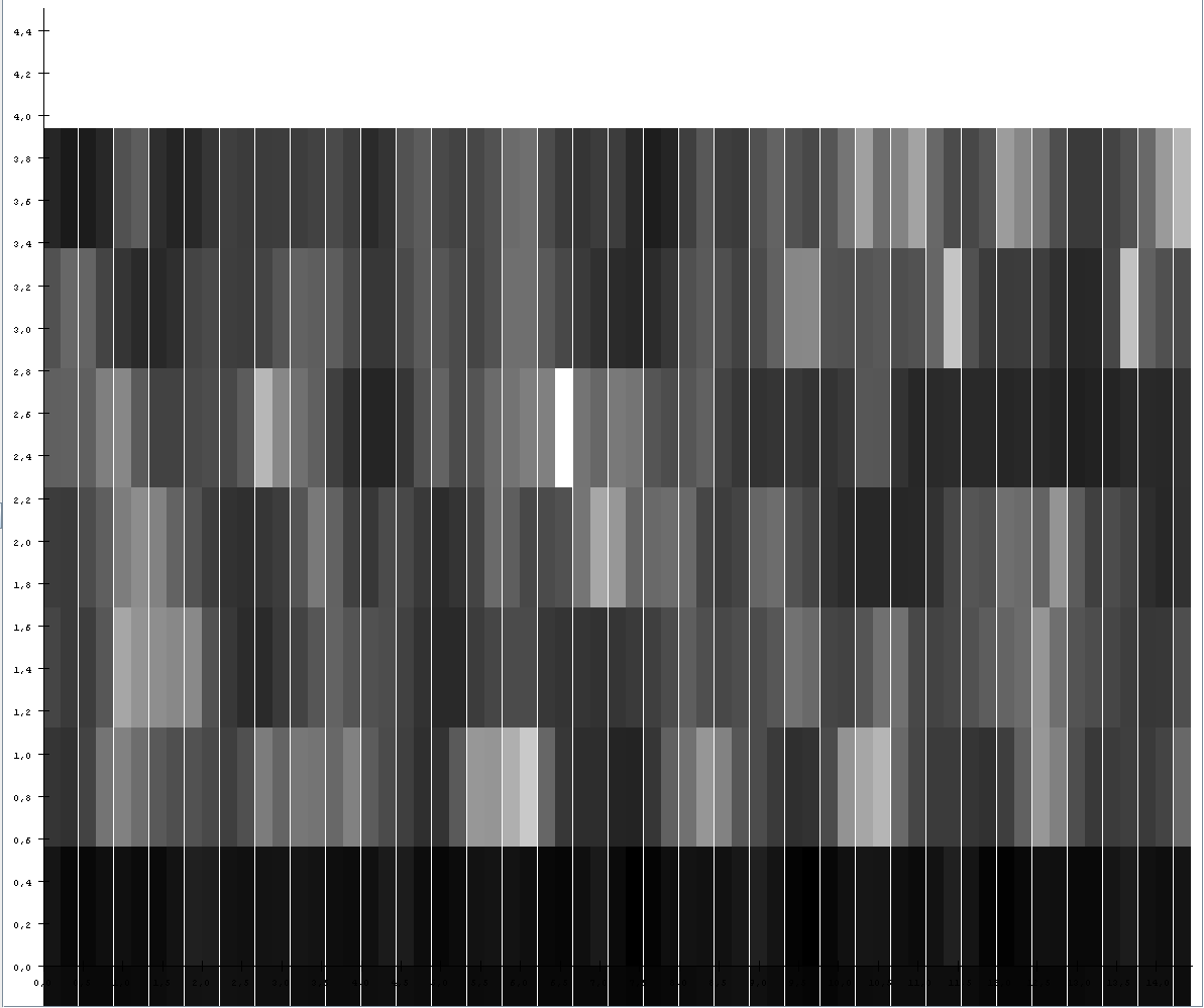
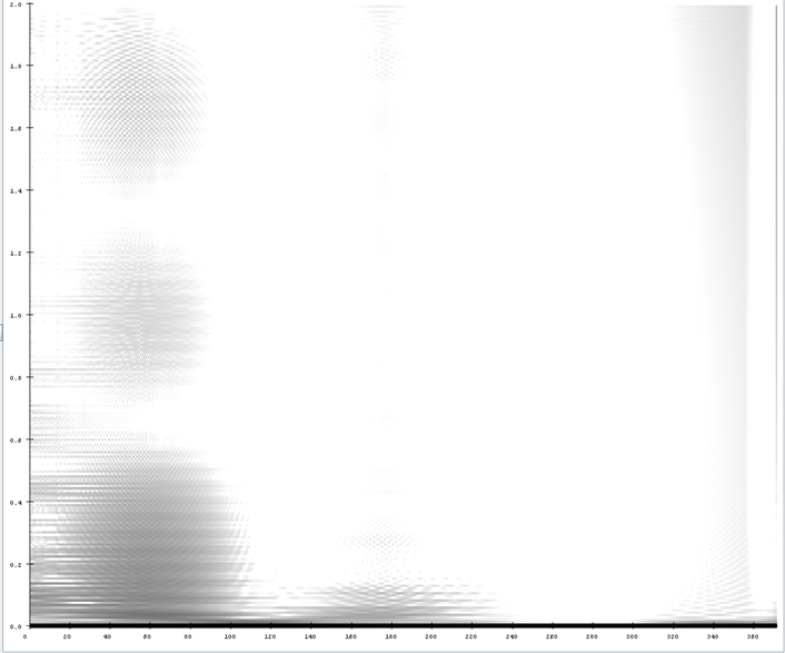
• Trace the Spectrogram of a Time Series
• Highlight periodicity in Time Series

Features

In the comparison between two maps belonging to NetCDF files, the map could not be defined at certain points. In the case of a layer on a GeoServer, the nearest neighbour algorithm is used by the GS itself to produce values at the required points. In the case of Thredds, the nearest neighbour must be applied programmatically by the client. I implemented some classes in the Ecological Engine Library wich perform basic signal processing, which will be used also in maps comparison.

In particular the following signal operations can now be applied:

signal reconstruction multi-signal analysis by means of summed spectrogram spectrogram calculation and display delta + double delta features center frequency calc. cepstral coefficients calc. spectrum frequency band cut filterbanks mel filterbanks

These are accompanied by the following transformation utilities: linear fequency to mel frequency frequency to index in Short-Time Fourier Transform transformation to and from Rapid Miner Example Set sinusoid signal generation inverse mel calc. sample to time and time to sample signal timeline generation index to time in spectrogram time to index in spectrogram

Figure 1.

Figure 2.

Figure 3.

Figure 4.

Figure 5.

Figure 6.