Signal Processing
Signal Processing is a set of facilities that aim to analyze signals, or measure time-varying or spatially varying physical quantities. It is part of the gCube system facilities for Data Mining and Processing. It is especially used in order to to discover seasonality and periodicity in time series of observations. Such observations can refer to catch statistics, species presence occurrence or environmental parameters modulations. The Signal Processing facilities are included in the Ecological Engine gCube library. Such library is responsible for hosting all the basic data processing and mining for on biological and environmental datasets. The Signal Processing facilities especially aim at facing the following issues:
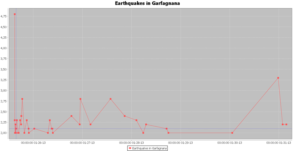
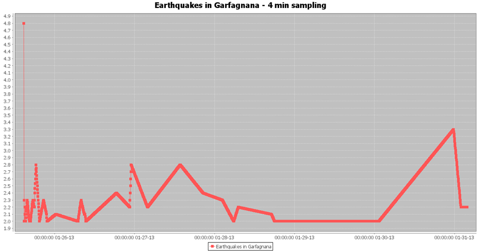
- Reconstruct a uniform sampled time series from a non-uniform time series
- Perform Short-Time Standard Fourier Analysis
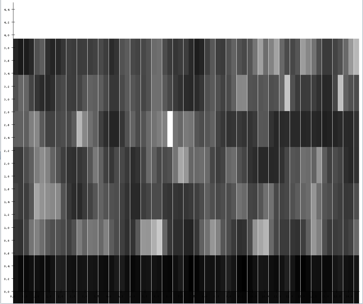
- Trace the Spectrogram of a Time Series
- Highlight periodicity in Time Series
Overview
Signal Processing is used in many ways by the gCube based e-Infrastructures. GIS layers, containing geographical information, can report the variations of some environmental parameters in time. Information can be stored in NetCDF files as well as on remote GeoServers. Geographical maps can contain information about environmental parameters distribution or species distributions, but these are usually not uniformly defined. At some point, in time and space, values can be missing. For such reasons, data mining techniques are put together with Signal Processing facilities by the Ecological Engine library, in order to fill the gaps, reconstruct signals and produce time-frequency analysis.
Features
The features supported by the Signal Processing facilities include:
- signal reconstruction: rebuilds a time series which is not uniformly sampled in time;
- spectrogram calculation and display: produces the spectrogram of a signal with the Short-Time Fourier Transform technique, according to a certain sampling frequency and time-window shift;
- multi-signal analysis by means of summed spectrogram: analyzes several synchronized signals and produces a spectrogram which is the sum of the single spectrograms;
- delta + double delta features: produces the delta and double delta features, correlated to the first and second derivative of the signal;
- center frequency calculation: calculated the central frequency in a filterbank;
- cepstral coefficients calculation: calculated the cepstral coefficients of a signal, which store much of the information contained in the signal;
- spectrum frequency band cut: cuts the signal spectrum according to a certain bandwidth;
- filterbanks: produces a filterbank for filtering the signal;
- mel filterbanks: builds a perceptually inspired filterbank based on the mel frequencies distribution.
A set of utilities are included in the Ecological Engine library in order to perform the above operations:
- linear fequency to mel frequency tranformation
- frequency to index in Short-Time Fourier Transform
- transformation to and from Rapid Miner Example Set
- sinusoid signal generation
- inverse mel calculation
- sample to time and time to sample conversions
- signal timeline generation
- index to time conversion for spectrograms
- time to index conversion for spectrograms
Experiments
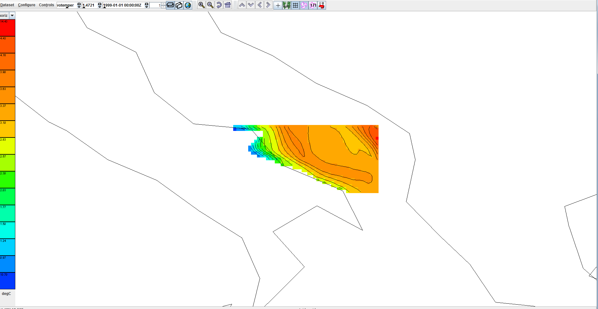
In the following experiments we give the idea of the transformations and processing that can be applied to signals with the Signal Processing facilities included in the 'Ecological Engine library. We selected a study area around Bari, Italy (ref. Fig. 1).
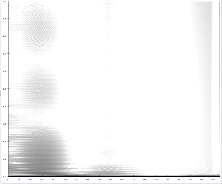
We then extracted the temperature time series from a point in that area with coordinates (17.59;41.37). We downloaded a NetCDF file from the MyOceans repository, which contained mean monthly variations for the temperature between 2000 and 2010. By using the geographical extraction facilities of gCube for the NetCDF files we extracted the time trend of the temperature. By using the Signal Processing facilities we produced the chart in Fig. 2.
