Difference between revisions of "Statistical Algorithms Importer: Create Project"
From Gcube Wiki
| Line 3: | Line 3: | ||
|} | |} | ||
| − | : | + | :This page explains how to create a project using Statistical Algorithms Importer(SAI) portlet. |
==Project Folder== | ==Project Folder== | ||
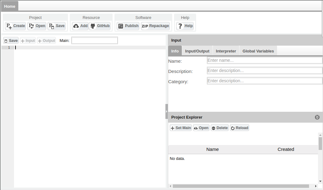
| − | : | + | :The fist step is to create or select an empty folder on the e-Infrastructure Workspace. Then, using the Create Project button in the main menu, the system creates an empty project in that folder. |
[[Image:StatisticalAlgorithmsImporter_CreateProject.png|thumb|center|800px|Create Project, SAI]] | [[Image:StatisticalAlgorithmsImporter_CreateProject.png|thumb|center|800px|Create Project, SAI]] | ||
==Import Resources== | ==Import Resources== | ||
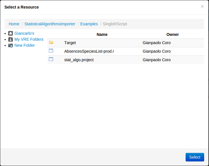
| − | :Any | + | :Any resource needed to run the script can be imported in the Project Folder. Resources cab be added either via the Workspace or using the Add Resource button in main menu, or dragging and dropping files in the folder window. |
| − | + | ||
[[Image:StatisticalAlgorithmsImporter_AddResource.png|thumb|center|800px|Add Resource, SAI]] | [[Image:StatisticalAlgorithmsImporter_AddResource.png|thumb|center|800px|Add Resource, SAI]] | ||
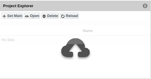
| − | : | + | :Thus, if the resource is on the user's local file system, (s)he can use the Drag and Drop facility, working also with multiple files. |
| − | [[Image:StatisticalAlgorithmsImporter_ProjectExplorerDND.png|thumb|center|800px| | + | [[Image:StatisticalAlgorithmsImporter_ProjectExplorerDND.png|thumb|center|800px|Adding resources with Drag and Drop, SAI]] |
==Set Main Code== | ==Set Main Code== | ||
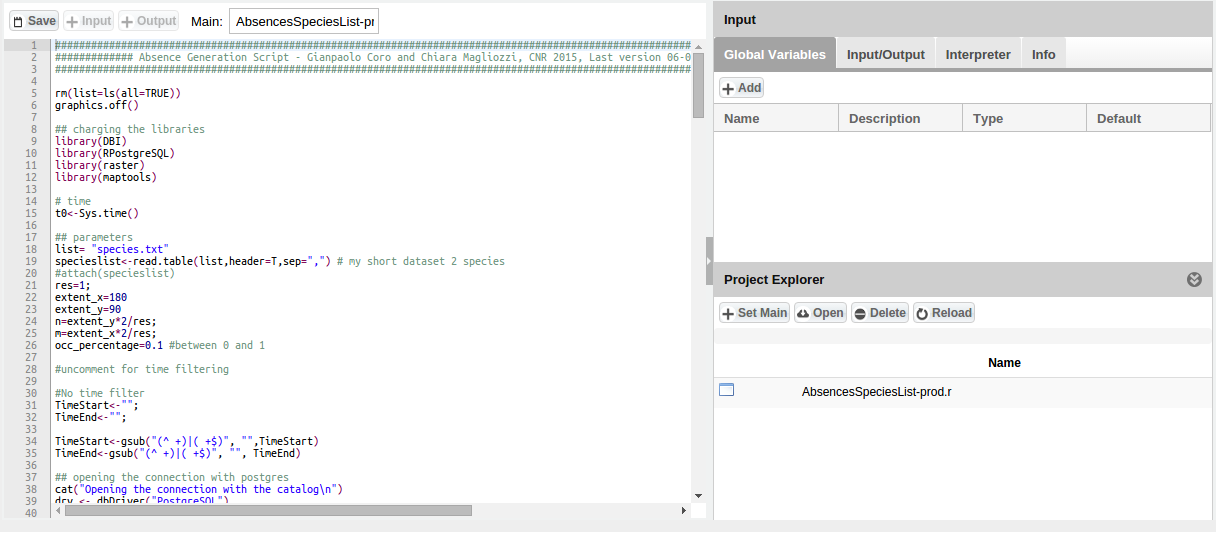
| − | :After | + | :After adding the scripts and resources, one of the script files should be indicated as Main code. The e-Infrastructure will run this code, which is supposed to import and orchestrate the other scripts. Indicating a script as Main code can be done by clicking the Set Main button in Project Explorer. The file will be loaded in the Editor. In this phase the system also reads possible annotations inside the script (e.g. WPS4R annotations). At this point, the user can change the code and save it using the Save button on the Editor panel. Alternatively, the user can also use Copy and Paste by writing the code directly in the editor and then save it, still using the Save button in Editor menu (A file name will be requested). |
| − | [[Image:StatisticalAlgorithmsImporter_MainCodeFull.png|thumb|center|800px|Set Main Code, SAI]] | + | [[Image:StatisticalAlgorithmsImporter_MainCodeFull.png|thumb|center|800px|Set Main Code facility, SAI]] |
==Input== | ==Input== | ||
Revision as of 14:22, 15 February 2016
- This page explains how to create a project using Statistical Algorithms Importer(SAI) portlet.
Project Folder
- The fist step is to create or select an empty folder on the e-Infrastructure Workspace. Then, using the Create Project button in the main menu, the system creates an empty project in that folder.
Import Resources
- Any resource needed to run the script can be imported in the Project Folder. Resources cab be added either via the Workspace or using the Add Resource button in main menu, or dragging and dropping files in the folder window.
- Thus, if the resource is on the user's local file system, (s)he can use the Drag and Drop facility, working also with multiple files.
Set Main Code
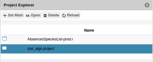
- After adding the scripts and resources, one of the script files should be indicated as Main code. The e-Infrastructure will run this code, which is supposed to import and orchestrate the other scripts. Indicating a script as Main code can be done by clicking the Set Main button in Project Explorer. The file will be loaded in the Editor. In this phase the system also reads possible annotations inside the script (e.g. WPS4R annotations). At this point, the user can change the code and save it using the Save button on the Editor panel. Alternatively, the user can also use Copy and Paste by writing the code directly in the editor and then save it, still using the Save button in Editor menu (A file name will be requested).
Input
- In this area you can set all input information to create software.
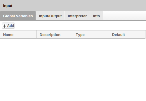
Global Variables
- In this panel you can add any useful Global Variable.
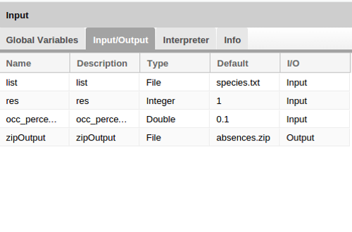
Input/Output
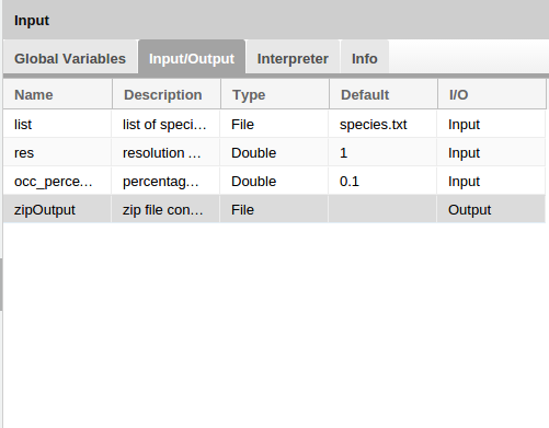
- For select input and output, you can select the row on the code in the Editor and than ckick Input or Output button on the Menu Editor. A new row is added to Input/Output list. Now if you need to you you can change your information by clicking on the row. At least one input is required for the project.
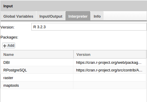
Interprer Info
- You can add Version and Packages informations in Interpreter Info panel. The version number is mandatory for the project.
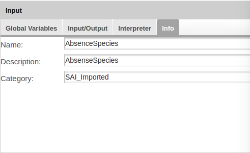
Project Info
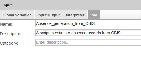
- Name and Description of project are mandatory, in addittion for Name special characters are not allowed. You can include a list of requested VREs for this algorithm.
Save Project
- You can save project by click on Save button in main menu. A file called stat_algo.project is add to Project Folder.
Use WPS4R Annotations
- If you import an R code with annotations, the system automatically try to fills the information into Input/Output panel and Project Info panel. Name of algorithm is mandatory in the annotations. This is an example of annotations:
############################################################################################################################
############# Absence Generation Script - Gianpaolo Coro and Chiara Magliozzi, CNR 2015, Last version 06-07-2015 ###########
############################################################################################################################

#52North WPS annotations
# wps.des: id = Absence_generation_from_OBIS, title = Absence_generation_from_OBIS, abstract = A script to estimate absence records from OBIS;

rm(list=ls(all=TRUE))
graphics.off()

## charging the libraries
library(DBI)
library(RPostgreSQL)
library(raster)
library(maptools)

# time
t0<-Sys.time()

## parameters
# wps.in: id = list, type = text/plain, title = list of species beginning with the speciesname header,value="species.txt";
list= "species.txt"
specieslist<-read.table(list,header=T,sep=",") # my short dataset 2 species
#attach(specieslist)
# wps.in: id = res, type = double, title = resolution of the analysis,value=1;
res=1;
extent_x=180
extent_y=90
n=extent_y*2/res;
m=extent_x*2/res;
# wps.in: id = occ_percentage, type = double, title = percentage of observations occurrence of a viable survey,value=0.1;
occ_percentage=0.1 #between 0 and 1

#uncomment for time filtering

#No time filter
TimeStart<-"";
TimeEnd<-"";

TimeStart<-gsub("(^ +)|( +$)", "",TimeStart)
TimeEnd<-gsub("(^ +)|( +$)", "", TimeEnd)

## opening the connection with postgres
cat("Opening the connection with the catalog\n")
drv <- dbDriver("PostgreSQL")
con <- dbConnect(drv, dbname="obis", host="obisdb-stage.vliz.be", port="5432", user="obisreader", password="0815r3@d3r")

cat("Analyzing the list of species\n")
counter=0;
overall=length(specieslist$scientificname)

cat("Extraction from the different contributors the total number of obs per resource id...\n")

timefilter<-""
if (nchar(TimeStart)>0 && nchar(TimeEnd)>0)
  timefilter<-paste(" where datecollected>'",TimeStart,"' and datecollected<'",TimeEnd,"'",sep="");

queryCache <- paste("select drs.resource_id, count(distinct position_id) as allcount from obis.drs", timefilter, " group by drs.resource_id",sep="")
cat("Resources extraction query:",queryCache,"\n")

allresfile="allresources.dat"
if (file.exists(allresfile)){
  load(allresfile)
} else{
  allresources1<-dbGetQuery(con,queryCache)
  save(allresources1,file=allresfile)
}

files<-vector()
f<-0
dir.create("data")

for (sp in specieslist$scientificname){
  f<-f+1
  t1<-Sys.time()
  graphics.off()
  grid=matrix(data=0,nrow=n,ncol=m)
  gridInfo=matrix(data="",nrow=n,ncol=m)
  outputfileAbs=paste("data/Absences_",sp,"_",res,"deg.csv",sep="");
  outputimage=paste("data/Absences_",sp,"_",res,"deg.png",sep="");

  counter=counter+1;
  cat("analyzing species",sp,"\n")
  cat("***Species status",counter,"of",overall,"\n")

  ## first query: select the species
  cat("Extraction the species id from the OBIS database...\n")
  query1<-paste("select id from obis.tnames where tname='",sp,"'", sep="")
  obis_id<- dbGetQuery(con,query1)
  cat("The ID extracted is ", obis_id$id, "for the species", sp, "\n", sep=" ")

  if (nrow(obis_id)==0) {
    cat("WARNING: there is no reference code for", sp,"\n")
    next;
  }

  ## second query: select the contributors
  cat("Selection of the contributors in the database having recorded the species...\n")
  query2<- paste("select distinct resource_id from obis.drs where valid_id='",obis_id$id,"'", sep="")
  posresource<-dbGetQuery(con,query2)

  if (nrow(posresource)==0) {
    cat("WARNING: there are no resources for", sp,"\n")
    next;
  }


  ## third query: select from the contributors different observations
  merge(allresources1, posresource, by="resource_id")-> res_ids

  ## forth query: how many obs are contained in each contributors for the species
  cat("Extraction from the different contributors the number of obs for the species...\n")
  query4 <- paste("select drs.resource_id, count(distinct position_id) as tgtcount from obis.drs where valid_id='",obis_id,"'group by drs.resource_id ",sep="")
  tgtresources1<-dbGetQuery(con,query4)
  merge(tgtresources1, posresource, by="resource_id")-> tgtresourcesSpecies

  ## fifth query: select contributors that has al least 0.1 observation of the species
  #### we have the table all together: contributors, obs in each contributors for at leat one species and obs of the species in each contributors
  cat("Extracting the contributors containing more than 10% of observations for the species\n")
  tmp <- merge(res_ids, tgtresourcesSpecies, by= "resource_id",all.x=T)
  tmp["species_10"] <- NA
  tmp$tgtcount / tmp$allcount -> tmp$species_10

  viable_res_ids <- subset(tmp,species_10 >= occ_percentage, select=c("resource_id","allcount","tgtcount", "species_10"))
  #cat(viable_res_ids)

  if (nrow(viable_res_ids)==0) {
    cat("WARNING: there are no viable points for", sp,"\n")
    next;
  }

  numericselres<-paste("'",paste(as.character(as.numeric(t(viable_res_ids["resource_id"]))),collapse="','"),"'",sep="")

  ## sixth query: select all the cell at 0.1 degrees resolution in the main contributors
  cat("Select the cells at 0.1 degrees resolution for the main contributors\n")
  query6 <- paste("select position_id, positions.latitude, positions.longitude, count(*) as allcount ",
                  "from obis.drs ",
                  "inner join obis.tnames on drs.valid_id=tnames.id ",
                  "inner join obis.positions on position_id=positions.id ",
                  "where resource_id in (", numericselres,") ",
                  "group by position_id, positions.latitude, positions.longitude, resource_id")
  all_cells <- dbGetQuery(con,query6)

  ## seventh query:  select all the cell at 0.1 degrees resolution in the main contributors for the selected species
  cat("Select the cells at 0.1 degrees resolution for the species in the main contributors\n")
  query7 <- paste("select position_id, positions.latitude, positions.longitude, count(*) as tgtcount ",
                  "from obis.drs",
                  "inner join obis.tnames on drs.valid_id=tnames.id ",
                  "inner join obis.positions on position_id=positions.id ",
                  "where resource_id in (", numericselres,") ",
                  "and drs.valid_id='",obis_id,"'",
                  "group by position_id, positions.latitude, positions.longitude")
  presence_cells<-dbGetQuery(con,query7)

  ## last query: for every cell in the sixth query if there is a correspondent in the seventh query I can put 1 otherwise 0
  data.df<-merge(all_cells, presence_cells, by= "position_id",all.x=T)
  data.df$longitude.y<-NULL
  data.df$latitude.y<-NULL
  data.df[is.na(data.df)] <- 0

  ######### Table resulting from the analysis
  pres_abs_cells <- subset(data.df,select=c("latitude.x","longitude.x", "tgtcount","position_id"))
  positions<-paste("'",paste(as.character(as.numeric(t(pres_abs_cells["position_id"]))),collapse="','"),"'",sep="")

  query8<-paste("select position_id, resfullname,digirname,abstract,temporalscope,date_last_harvested",
                "from ((select distinct position_id,resource_id from obis.drs where position_id IN (", positions,
                ") order by position_id ) as a",
                "inner join (select id,resfullname,digirname,abstract,temporalscope,date_last_harvested from obis.resources where id in (",
                numericselres,")) as b on b.id = a.resource_id) as d")

  resnames<-dbGetQuery(con,query8)
  #sorting data df
  pres_abs_cells<-pres_abs_cells[with(pres_abs_cells, order(position_id)), ]

  nrows = nrow(pres_abs_cells)
  ######## FIRST Loop inside the rows of the dataset
  cat("Looping on the data\n")
  for(i in 1: nrows) {
    lat<-pres_abs_cells[i,1]
    long<-pres_abs_cells[i,2]
    value<-pres_abs_cells[i,3]
    resource_name<-paste("\"",paste(as.character(t(resnames[i,])),collapse="\",\""),"\"",sep="")#resnames[i,2]
    k=round((lat+90)*n/180)
    g=round((long+180)*m/360)
    if (k==0) k=1;
    if (g==0) g=1;
    if (k>n || g>m)
      next;
    if (value>=1){
      if (grid[k,g]==0){
        grid[k,g]=1
        gridInfo[k,g]=resource_name
      }
      else if (grid[k,g]==-1){
        grid[k,g]=-2
        gridInfo[k,g]=resource_name
      }
    }
    else if (value==0){
      if (grid[k,g]==0){
        grid[k,g]=-1
        #cat("resource abs",resource_name,"\n")
        gridInfo[k,g]=resource_name
      }
      else if (grid[k,g]==1){
        grid[k,g]=-2
        gridInfo[k,g]=resource_name
      }

    }
  }
  cat("End looping\n")

  cat("Generating image\n")
  absence_cells<-which(grid==-1,arr.ind=TRUE)
  presence_cells_idx<-which(grid==1,arr.ind=TRUE)
  latAbs<-((absence_cells[,1]*180)/n)-90
  longAbs<-((absence_cells[,2]*360)/m)-180
  latPres<-((presence_cells_idx[,1]*180)/n)-90
  longPres<-((presence_cells_idx[,2]*360)/m)-180
  resource_abs<-gridInfo[absence_cells]

  absPoints <- cbind(longAbs, latAbs)
  absPointsData <- cbind(longAbs, latAbs,resource_abs)

  if (length(absPoints)==0)
  {
    cat("WARNING no viable point found for ",sp," after processing!\n")
    next;
  }
  data(wrld_simpl)
  projection(wrld_simpl) <- CRS("+proj=longlat")
  png(filename=outputimage, width=1200, height=600)
  plot(wrld_simpl, xlim=c(-180, 180), ylim=c(-90, 90), axes=TRUE, col="black")
  box()
  pts <- SpatialPoints(absPoints,proj4string=CRS(proj4string(wrld_simpl)))

  ## Find which points do not fall over land
  cat("Retreiving the poing that do not fall on land\n")
  pts<-pts[which(is.na(over(pts, wrld_simpl)$FIPS))]
  points(pts, col="green", pch=1, cex=0.50)
  datapts<-as.data.frame(pts)
  colnames(datapts) <- c("longAbs","latAbs")

  abspointstable<-merge(datapts, absPointsData, by.x= c("longAbs","latAbs"), by.y=c("longAbs","latAbs"),all.x=F)


  header<-"longitude,latitude,resource_id,resource_name,resource_identifier,resource_abstract,resource_temporalscope,resource_last_harvested_date"
  write.table(header,file=outputfileAbs,append=F,row.names=F,quote=F,col.names=F)

  write.table(abspointstable,file=outputfileAbs,append=T,row.names=F,quote=F,col.names=F,sep=",")
  files[f]<-outputfileAbs
  cat("Elapsed:  created imaged in ",Sys.time()-t1," sec \n")
  graphics.off()
}

# wps.out: id = zipOutput, type = text/zip, title = zip file containing absence records and images;
zipOutput<-"absences.zip"
zip(zipOutput, files=c("./data"), flags= "-r9X", extras = "",zip = Sys.getenv("R_ZIPCMD", "zip"))

cat("Closing database connection")
cat("Elapsed:  overall process finished in ",Sys.time()-t0," min \n")
dbDisconnect(con)
graphics.off()
File:AbsencesSpeciesList prod annotated.zip
- This is the result in SAI:
