Difference between revisions of "Legacy applications Biological Observations Enrichment"
Julien.barde (Talk | contribs) (→2.2.3 Method for biological observation locations given by lines) |
|||
| (6 intermediate revisions by one other user not shown) | |||
| Line 1: | Line 1: | ||
| + | [[Category: gCube Spatial Data Infrastructure]][[Category:TO BE REMOVED]] | ||
| + | |||
== 1. Main Goal : == | == 1. Main Goal : == | ||
| − | We aim at adding some values related to environmental parameters observations (taken from datasets which are coverages managed in multi-dimensionsal raster data format: netCDF-CF or HDF or any [http://gdal.org/formats_list.html | + | We aim at adding some values related to environmental parameters observations (taken from datasets which are coverages managed in multi-dimensionsal raster data format: netCDF-CF or HDF or any gdal data formats [http://gdal.org/formats_list.html]) to existing biological observations which are georeferenced with various geometries / Features (points, lines, polygons…) and managed in vector formats (in spatial RDBMS or any ogr data formats [http://www.gdal.org/ogr_formats.html]: shapefiles..). This process has thus to deal with usual '''rasterization''' and '''vectorization''' issues which are not obvious for many scientists in ecology. |
Depending on data sources, this kind of process has to take into account some cases where the coverages expected to supply additionnal environmental observations are not available for some given dates and given locations (cloud cover…). When there is a lack of coverage, data search has to be extended to a set of coverages which are within a given spatio-temporal frame (through '''buffers'''). | Depending on data sources, this kind of process has to take into account some cases where the coverages expected to supply additionnal environmental observations are not available for some given dates and given locations (cloud cover…). When there is a lack of coverage, data search has to be extended to a set of coverages which are within a given spatio-temporal frame (through '''buffers'''). | ||
Moreover, according to the data types and the users, depending on the kinds of biological and environmental parameters, the spatio-temporal distance between Features and Coverages used to collect a set of raster cells as well as '''statistical methods''' which can be applied to calculate missing values will differ. The ability to tune the execution of each process with a set of input parameters is key. However default methods are used for users who don’t know how to manage underlying spatial analysis. | Moreover, according to the data types and the users, depending on the kinds of biological and environmental parameters, the spatio-temporal distance between Features and Coverages used to collect a set of raster cells as well as '''statistical methods''' which can be applied to calculate missing values will differ. The ability to tune the execution of each process with a set of input parameters is key. However default methods are used for users who don’t know how to manage underlying spatial analysis. | ||
| Line 77: | Line 79: | ||
See alternative statistical treatments described in section 3.3 | See alternative statistical treatments described in section 3.3 | ||
| + | |||
| + | |||
| + | = 3 Alternative methods = | ||
| + | |||
| + | To be done... | ||
| + | The goal here is to get advices from researchers to enable a set of alternative methods covering various use cases for biological observations (biodiversity, fisheries...) and environmental data (satellites and model outputs will be the priority before dealing, if possible, with in situ data..) | ||
| + | |||
| + | |||
| + | === 3.1 Temporal buffers === | ||
| + | |||
| + | |||
| + | ==== 3.1.1 2D: Latitude and Longitude ==== | ||
| + | [[File:Biological_observations_enrichment_figure_7.jpg|center|thumb|600px|Figure 7: .....]] | ||
| + | |||
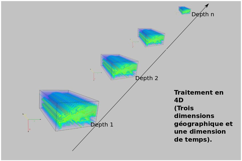
| + | ==== 3.1.2 3D: Depth ==== | ||
| + | |||
| + | [[File:Biological_observations_enrichment_figure_8.jpg|center|thumb|600px|Figure 8: .....]] | ||
| + | |||
| + | === 3.2 Spatial buffers === | ||
| + | |||
| + | |||
| + | === 3.3 Statistical methods === | ||
Latest revision as of 18:28, 6 July 2016
Contents
1. Main Goal :
We aim at adding some values related to environmental parameters observations (taken from datasets which are coverages managed in multi-dimensionsal raster data format: netCDF-CF or HDF or any gdal data formats [1]) to existing biological observations which are georeferenced with various geometries / Features (points, lines, polygons…) and managed in vector formats (in spatial RDBMS or any ogr data formats [2]: shapefiles..). This process has thus to deal with usual rasterization and vectorization issues which are not obvious for many scientists in ecology. Depending on data sources, this kind of process has to take into account some cases where the coverages expected to supply additionnal environmental observations are not available for some given dates and given locations (cloud cover…). When there is a lack of coverage, data search has to be extended to a set of coverages which are within a given spatio-temporal frame (through buffers). Moreover, according to the data types and the users, depending on the kinds of biological and environmental parameters, the spatio-temporal distance between Features and Coverages used to collect a set of raster cells as well as statistical methods which can be applied to calculate missing values will differ. The ability to tune the execution of each process with a set of input parameters is key. However default methods are used for users who don’t know how to manage underlying spatial analysis.
We will enrich step by step a process (written in R) whose structure is made of functions in charge of:
- 1) rasterization / vectorization issues,
- 2) temporal and spatial buffers to collect additional values (populations of pixels) when expected ones are missing,
- 3) statistical methods to analyze the characteristics of the population of pixels returned by function 2 and calculate a set of values (mean value, standard deviation…).
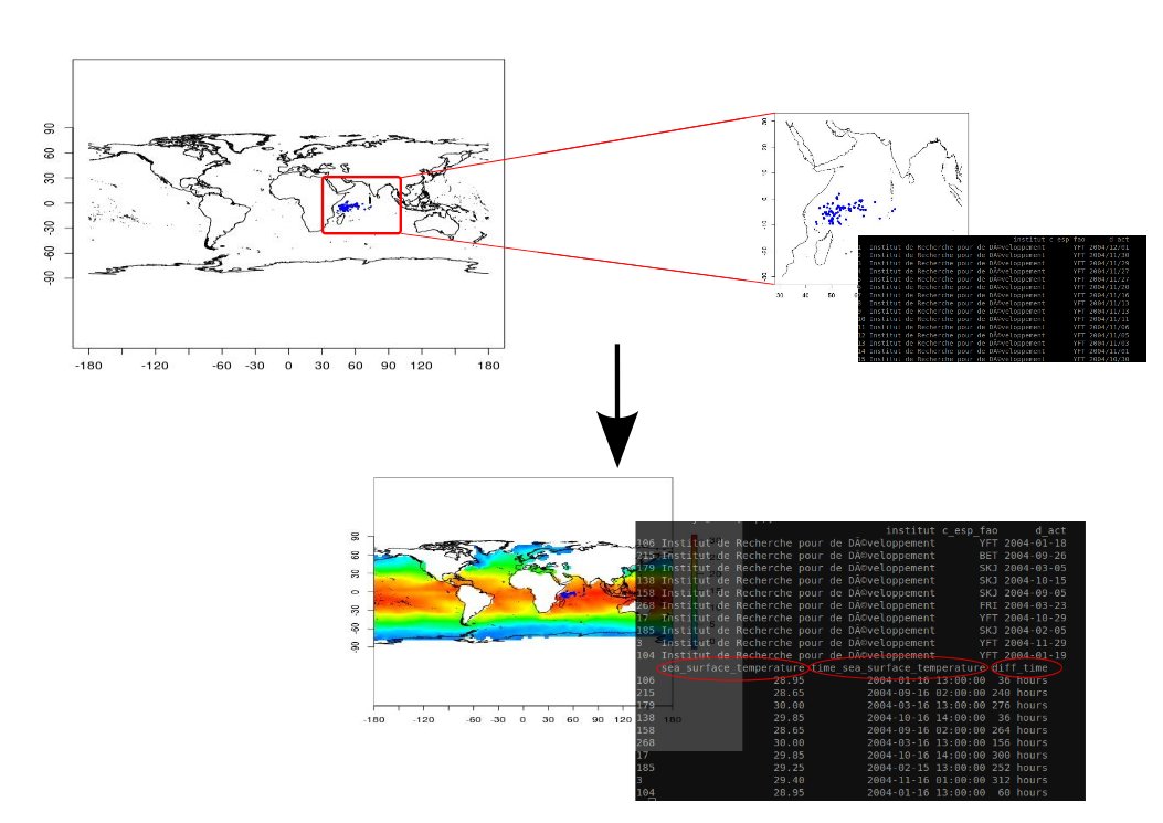
The Figure 1 gives an example of biological observations which are enriched with environmental parameters. In this case points describing fishing operations are extracted from the BALBAYA database managed in a spatial RDBMS (Postgres & Postgis). The user indicates the URL giving access to a netCDF-CF file (through OPeNDAP protocol) to extract values related to the SST variable.
In the next sections, we describe the possible options to collect environmental parameters in different ways and apply different kinds of calculation methods (mean value with or without ponderation, error bar…).
2. Default options of the process
2.1 Default function for temporal buffer:
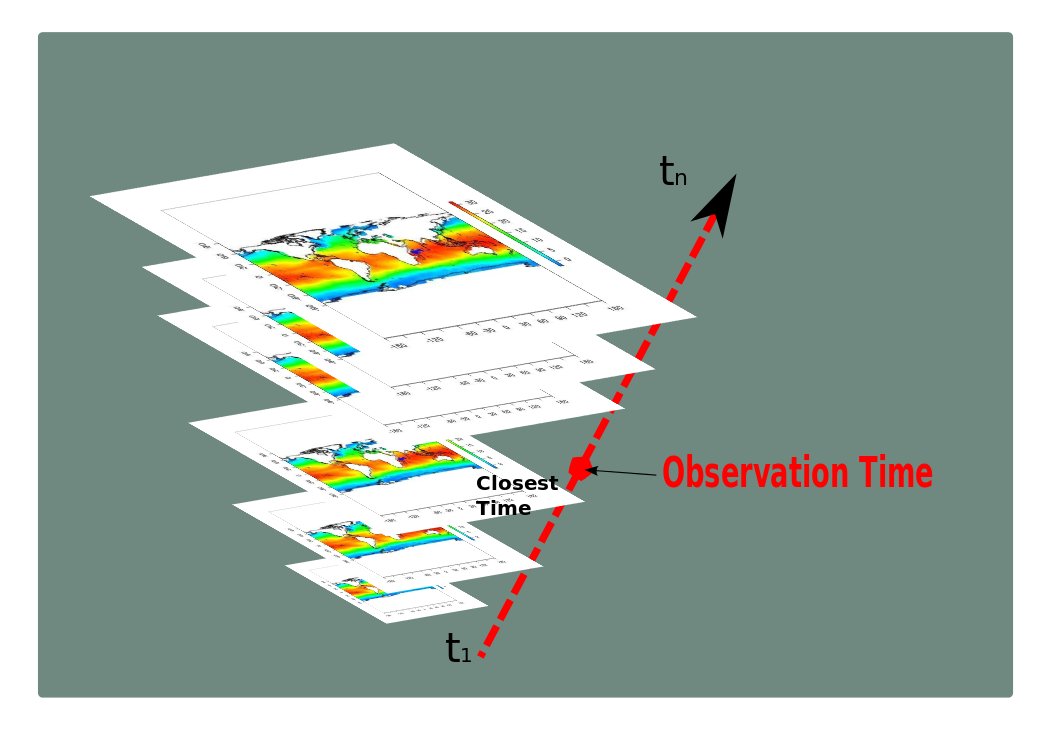
By default, this R script executes a simple temporal buffer 'ClosestTime' which collects a set of coverages (datasets) for which the temporal distance (for given time units, days by default) is the closest from each geometry related to a biological observation (brought by users).
2.2 Default function for spatial buffer:
Whatever the type of features, it is required to rasterize the location of each biological observation to extract the values of environmental parameters in the proper cells of coverages which are stored in netCDF files. To achieve this we use different spatial analysis functions according the type of geometry for each feature (points, lines, polygons).
2.2.1 Method for biological observation locations given by points
In this method, we first search the location (“longitude – latitude”) of points related to biological observations et we harvest environmental data values which are:
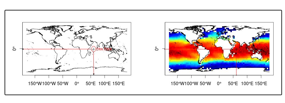
- either exactly at this location (matching cells in the raster file) as shown in Figure 2,
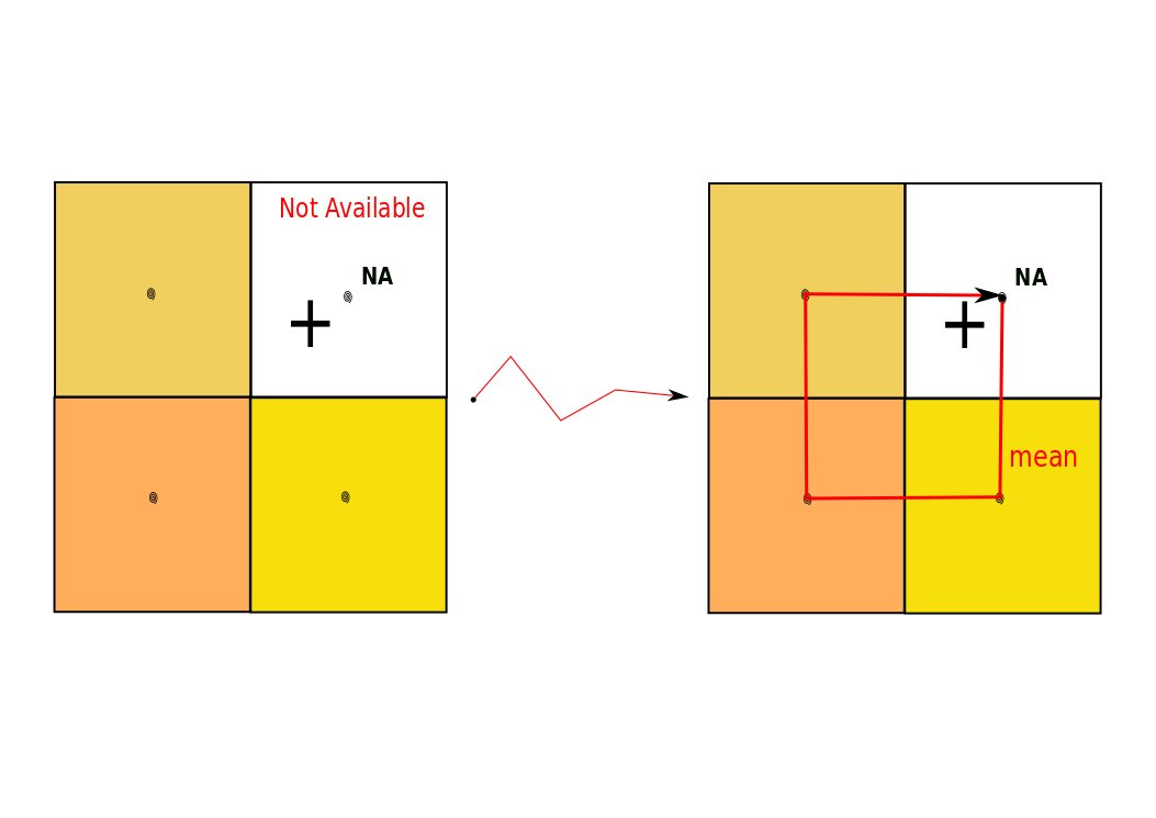
- or (no values / NaN in matching cells) we enlarge the search area by using differents kinds of spatial buffer:
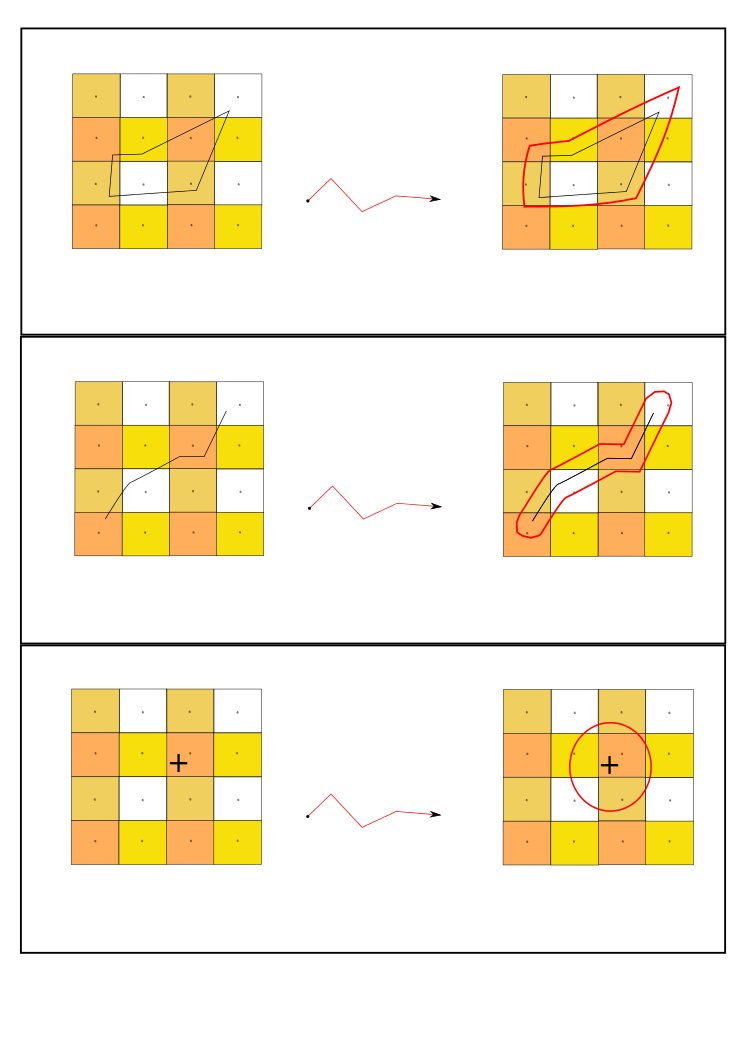
- the default spatial buffer is illustrated in Figure 4: we collect the values of the 4 closest pixels,
- alternative methods for spatial buffers are described in section 3.2.1
2.2.2 Method for biological observation locations given by polygons
For this type of geometry, we extract a population of pixels / cells which are located in rasterized biological observations areas. To achieve this, we aim at proposing different methods:
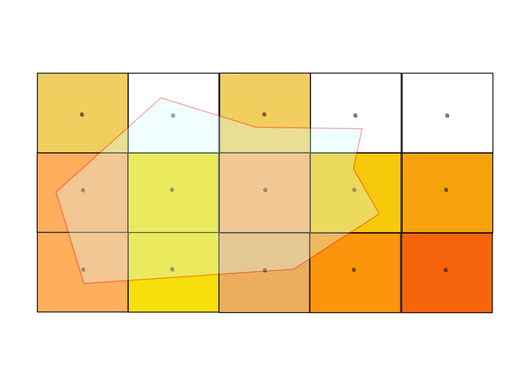
- default method (illustration in Figure 5): the default spatial analysis enables to collect the pixels which are within or overlapping the observation area. For each cell of this pixel population, a P factor (weight for ponderation) is returned:
- P = 1 for pixels within the polygon.
- P ∊ ]0,1[ for pixels only overlapping the polygon.
- alternative methods for spatial buffers are described in section 3.2.2
2.2.3 Method for biological observation locations given by lines
For this type of geometry, we apply the same method as the one used for polygons: we collect all the pixels crossed by the lines related to observations.
Once temporal and spatial processes have been applied, a population of pixels is extracted from netCDF-CF and are thereafter forwarded to statistical functions.
2.3 Default statistical function for the calculation of the additional value to enrich the biological observation
By default, the biological observation is enriched with the average weighted by the spatio-temporal distance between the biological observation and each pixel of the population (within or overlapping the biological observation location). In this default method, the functions returns for each geometry, the completeness of data (rate between cells with available values among all possible ones: data + Nan). This last value is meant to help users to appreciate the quality of the environmental data which is returned to enrich the biological observation (confidence indicator).
M = ∑ ⁿαimi ⁄ ∑ⁿαi where:
- M = {m₁,m₂,...,mᵤ} : are the values of environmental data for the pixels within or overlapping the biological observations locations.
- α = {α₁α₂,...,αᵤ} : the weight (>o) corresponding to each pixelVoir les autres .
See alternative statistical treatments described in section 3.3
3 Alternative methods
To be done... The goal here is to get advices from researchers to enable a set of alternative methods covering various use cases for biological observations (biodiversity, fisheries...) and environmental data (satellites and model outputs will be the priority before dealing, if possible, with in situ data..)
